Mathematical background

What are flags?

Let \( \mathbb{RP}^2\) be the real projective plane. A flag is a tuple \((p, l)\) consisting of a point \(p\) in \(\mathbb{RP}^2\) and a projective line \(l\) containing the point. Most of the time, we will only be considering a special case, positive tuples of flags. In fact, a lot geometric ideas only make sense in this case. In this case the polygon spanned by the points of the flags lies inside the polygon spanned by the intersection points of the lines. We denote the set of positive \(n\)-tuples of flags by \(\mathcal{F}^n_+\).

The application checks whether the tuple of flags you drew is positive and alerts you if not.

The action of the projective linear group \(\mathbf{PGL}(3,\mathbb{R})\) on \(\mathbb{RP}^2\) descends to an action on \(\mathcal{F}^n_+\).

Transformations of flag tuples

Defining the eruption flow

The eruption flow is a flow on positive triples of flags which doesn't come from the action of \(\mathbf{PGL}(3,\mathbb{R})\). Nevertheless, it commutes with the action, and therefore also induces a flow on the orbit space. We define it as follows.

Let \((p_i,l_i)_{i=1,2,3}\in\mathcal{F}^3_+\) be a triple of flags. It is equivalent to a pair of nested triangles \(\Delta=(p_1, p_2, p_3)\) and \(\Delta'=(q_1, q_2, q_3)\) as can be seen in the figure below. This induces three quadrilaterals \(Q_1, Q_2\) and \(Q_3\).

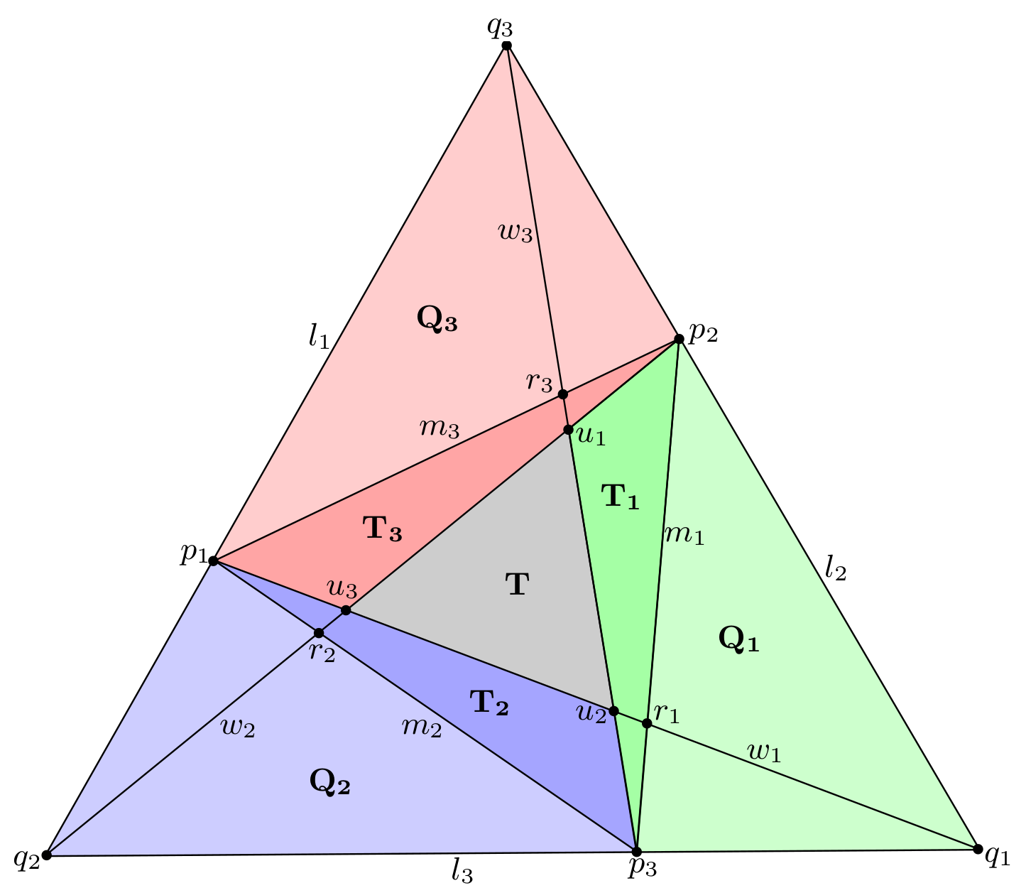
The flow is now defined by deforming each quadrilateral \(Q_i\) with a different element of \(\mathbf{PGL}(3,\mathbb{R})\), namely

\[ g_1(t) =\begin{pmatrix}1 & 0 & 0\\0 & e^{\tfrac{t}{3}} & 0\\0 & 0 & e^{-\tfrac{t}{3}} \\ \end{pmatrix}, \quad g_2(t) = \begin{pmatrix} e^{-\tfrac{t}{3}} & 0 & 0\\ 0 & 1 & 0\\ 0 & 0 & e^{\tfrac{t}{3}}\\ \end{pmatrix},\]

\[\quad g_3(t) =\begin{pmatrix}e^{\tfrac{t}{3}} & 0 & 0\\ 0 & e^{-\tfrac{t}{3}} & 0\\ 0 & 0 & 1\\ \end{pmatrix}\]

where all matrices are written in a basis given by representatives of \(q_1, q_2\) and \(q_3\). In fact, this transformation leaves the points \(q_i\) invariant. The transformed points \(p_i(t)\) remain on the lines \(l_i\), so the transformation gives us a pair of nested triangles \(\Delta(t),\Delta'(t)\) equivalent to a triple of flags, as can be seen in the figure above.

The points \(u_i\) are the inner triangle in the application. The points \(p_i\) are the middle triangle. The lines connecting \(p_i\) and \(q_i\) are the helper lines.

Other transformations

The eruption flow can be easily generalized to larger numbers of flags by simply dividing the tuple of flags into triangles and applying the eruption flow to every single one. In this case, we will have a choice though, we could run through each triangle by changing the parameter \(t\) in positive or in negative direction.

For this reason, we have included eruption flow (-/+) and eruption flow (+/+) in the application.

By similar divisions of the polygon and applying similar matrices, we obtain two more transformations: the bulge flow and the shear flow in the case of 4-tuples of flags.

The shear flow has one specialty. One of his points will remain on a fixed ellipse at all times of the transformation, which can also be seen in the application.

Convex sets

In fact, a tuple of four flags defines two nested quadrilaterals: The outer quadrilateral is spanned by the intersection points \(q_i\) of the lines, the inner quadrilateral is spanned by the \(p_i\). We can construct a convex set from the inner quadrilateral by reflecting it along each of it sides. We repeat this procedure up to infinity. By reflection, we mean a special kind of projective reflection: Imagine you are standing on train tracks and seeing a point \(v\) at the horizon where the parallel tracks meet. Imagine the quadrilateral lying on the ground. If you reflect it along one of its sides \(l\), it will look different than its mere mirror image. This is due to the perspective. As a mathematical formula, we write this projective reflection as

\[R(x) = x - l(x)v\]

where \(l(\cdot)\) is the linear form that defines the projective line \(l\).

Visualizing the projective plane

The projective plane \(\mathbb{RP}^2\) is an abstract mathematical object that has different equivalent definitions. How do we visualize this space?

Define the projective plane as the space of all straight lines through the origin of \(\mathbb{R}^3\). We can visualize a big part of this space by projecting those lines to a plane: Choose a plane that has distance 1 from the origin. Every line that intersects with the plane will be represented by the intersection point, so we have a two-dimensional visualization of a chunk of \(\mathbb{RP}^2\). The lines that don't intersect with the plane (as they are parallel to the plane) are the infamous "points at infinity".

The Projection Plane setting in the application is simply the normal vector of this plane.

Sources

The mathematical information on this site is due to

Wienhard, A.; Zhang, T. (2017). Deforming convex real projective structures. math.GT; arXiV 1702.00580.